NN in CMS
Introduction
The very basic idea of any multivariate analysis or supervised machine learning (ML) tool for classification is to make a more optimal use of a set of discriminating variables xi than each of these variables, either individually or two-by-two or three-by-three, which is the highest dimension a human can geometrically represent. An ML can at least make a more optimal chain of decisions via 1-dimensional (1D) cuts (like Boosted Decision Trees - BDTs) than human based 1D or 2D decisions. This is exactly what BDTs do, where each tree applies an ensemble of 1D cuts, and where the forest of trees effectively applies cuts of higher dimensions. It can also exploit the differences of correlation among the input variables xi for S and B events (like Deep Neural Networks - NNs).
In this tutorial, we will first go through the basic ideas of a NN, then cover its different metrics, and then cover how events/samples should be treated. In each section, we will provide code snippets as to illustrate the practice of each covered point. To not overload the flow of the tutorial, these pieces of code will be just snippets, and full example codes will be provided in the last section.
The basics of a NN
In this section, we will cover the basic concepts of a Neural Network (NN) classifier. First, we will cover the quantity which is minimized and is guiding the training of a NN, quantity which can also be used by other classifiers. Then we will cover the specifics of a NN classifier, namely its architecture and how one builds its output discriminator as function of the input variables. We will then cover how a NN is trained, and go over the activation functions of a NN. Finally, we will provide code snippets illustrating the mentioned functionalities.
Loss functions: binary & multi-class
When classifying events, we need to optimize a quantity which quantifies our classification; this quantity can be a loss function. If we are dealing with a binary classification of Signal (S) versus Background (B), we need a measure of how much we have classified signal events as S, and background events as B. The binary cross-entropy, which is one such quantity, is one of the loss functions used for binary studies, and is averaged over N events:
where:
- \(z(i)\) is the true classification: it is 1 for S, and 0 for B; this can be viewed as the tag of the event, ie. the prior knowledge that we provide to the classifier for this latter to know which event is S or B.
- \(y(i)\) is the classifier's output, with its value between 0 and 1, ie. its prediction for whether an event is S(1) or B(0).
\(L\) is reflective of the morphology of the classifier: the measure of the classification, itself a function of the separation achieved by the classifier. In equation (1), the first and second terms are "signal" and "background" term respectively. Indeed:
- \(L = - \frac{1}{N} \times \Sigma_{i=1}^{N} ln(y(i))\). If the prediction is S: \(y(i) \rightarrow 1\), then we have \(L \rightarrow 0\).
- \(L = - \frac{1}{N} \times \Sigma_{i=1}^{N} ln(1 - y(i))\). If the prediction is B: \(y(i) \rightarrow 0\), then we have \(L \rightarrow 0\).
The general, ie. multi-class, cross-entropy is given by:
where \(j\) is the index of \(m\) different classes. Eq. (1) is easily obtained by considering \(m=2\), and considering that for each event \(i\), we have \(z_1 + z_2 = 1\) and \(y_1 + y_2 = 1\).
It has to be noted that Keras, an open-source library in Python for artificial neural networks, minimizes a slightly different loss function. For example, for binary classification, the cross-entropy that Keras minimizes is given by:
where \(w_i\) is the event weight, reflecting the number of events in the sample, cross section, etc; it takes into account the (signal and background) samples, both in their shape (through bins of a distribution) and normalization. Therefore, to have a numerically balanced problem to solve, the weights should be made to be comparable:
We will cover more this latest aspect in the subsection "Event balancing". Finally, it should be noted that for NNs performing tasks other than classification, loss functions different from cross-entropy are minimized. For example, for the case of a NN performing a regression, the minimized loss function is often the Mean Squared Error.
Architecture & weights
In a NN, the information of the \(n\) input variables \(x_i\) is propagated to different nodes as illustrated in figure 1, where we represent a NN with one hidden layer of \(m\) nodes. The information is propagated from the input nodes to the output node(s) via the hidden layer(s), representing the foward propagation of the NN. In this example, there is only output node. In the case of a multi-class NN, there is as much nodes as classes for classification.
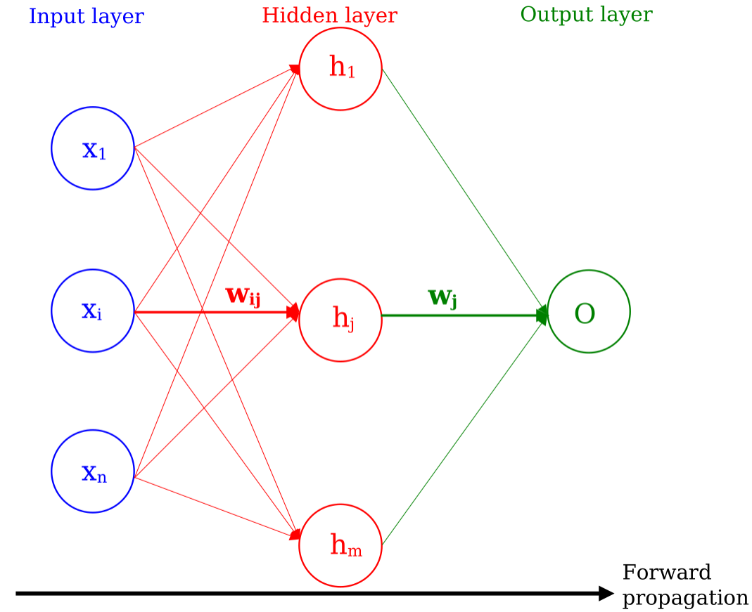
Figure 1
Here, each input node \(i\) sends the same input variable \(x_i\) to all nodes of the hidden layer. Overall, the NN is fully connected, meaning that each node of a given layer has a connection with all nodes of the subsequent layer. The lines, ie. the numerical connections, between the nodes are the weights \(w\), all different from one another, and are updated during the training of the NN (see section on learning). Higher/Lower weights indicate a stronger/weaker influence of one neuron on another. The hidden layers of the NN can be viewed as functions of the variables/nodes of the previous layer.
In the case of a NN with one hidden layer, the output discriminant \(y\) of a NN at the output layer is given as a function of input variables \(x_i\):
where \(w_{ij}\) is the weight between node \(i\) of a layer and node \(j\) of another layer, \(w_j\) is the weight between node \(j\) of penultimate layer and the output. \(g\) is the activation function (see section on activation functions) operating at each node \(h_j\) of the hidden layer. As such, y retains the information about the input variables plus a set of weights optimized to minimize the cross-entropy loss.
Learning/Training of a NN
The NN is trained iteratively on the (training) data to adjust the weights, aiming to find their optimal values that minimize the loss, ie. minimize the difference between its predictions and the true values. This is done in the backward propagation step of the training, as illustrated in the figure below. The full iteration of a forward- & backward-propagation is called an epoch, ie. epoch in the training of the NN.
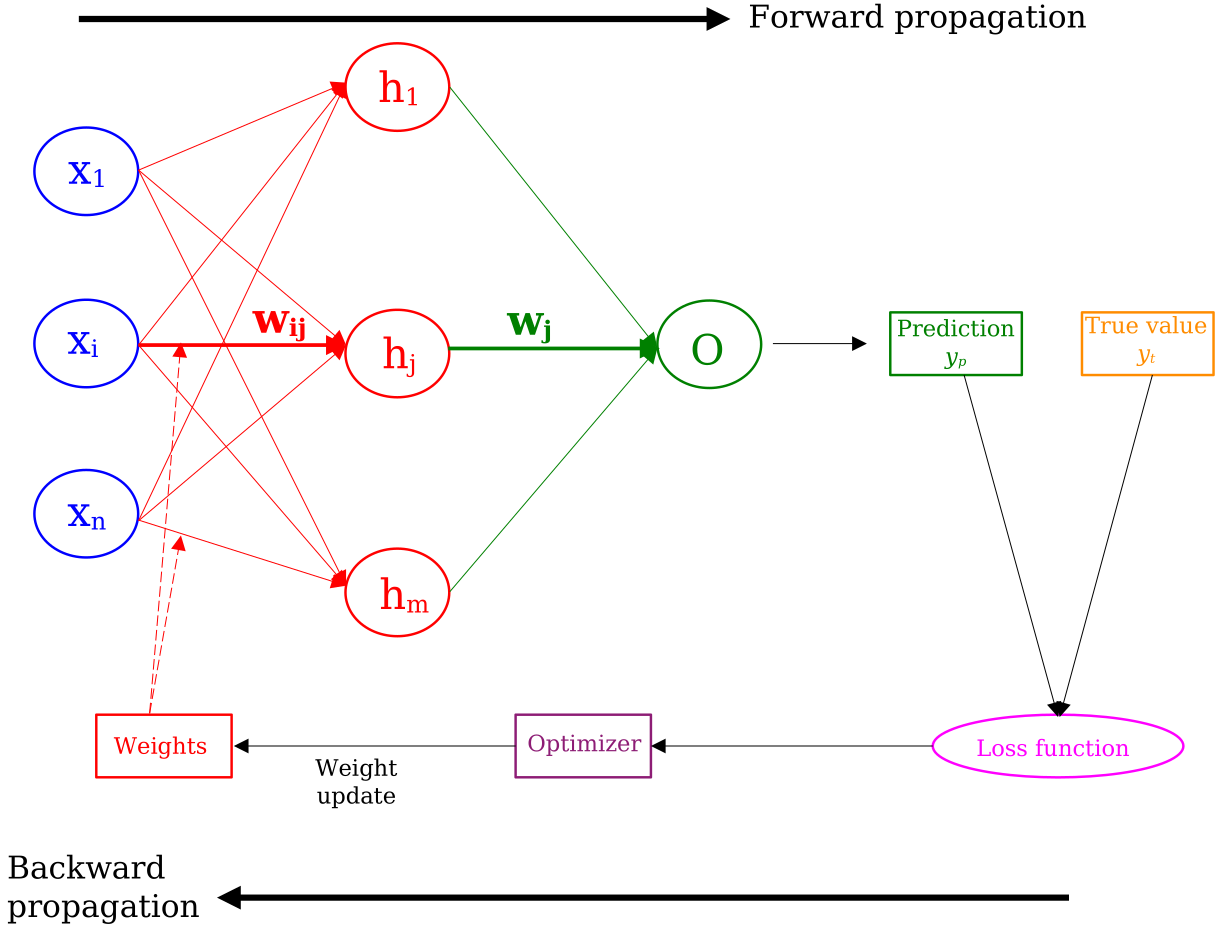
Figure 2
The prediction of the NN for an event \(y_p\) is compared with the true value \(y_t\), comparison upon which the loss value is calculated. This latter value is in turn fed to the optimizer, which updates the weights, injecting them back in the forward propagation part of the training. We cover the two most known optimizers in the two subsections below.
Gradient descent
The equation giving the evolution of the weights \(w_{tij}\) at epoch \(t\), is:
where \(R\) and \(D\) are the learning and decay rates, respectively. \(R\) is usually tested in the \([10^{-5},10^{-2}]\) interval. \(\Delta w^t_{ij}\) is the partial derivative (versus \(w\)) of the back-propagation between two epochs:
This gradient gives the direction of the steepest increase of the loss function, and the learning rate \(R\) controls the step size taken during an update in that direction. By moving in the opposite direction of the gradient, the algorithm iteratively adjusts the weights to reduce the error and improve the NN's performance. Let us explain this latter point more explicitly. The derivative of Eq. (6), within Eq. (5), points in the direction where the loss function \(L_K\) decreases the most:
- If \(\frac{\delta L_K}{\delta w} \geq 0\): \(L_K\) is increasing, then \(w_{ij}^{t+1} \leq w_{ij}^t\), thus weights will decrease and one can only have \(\frac{\delta L_K}{\delta w} \sim 0\).
- If \(\frac{\delta L_K}{\delta w} \leq 0\): \(L_K\) is decreasing, meaning that there is less cross-entropy, thus \(L_K \rightarrow 0\), thus: \(\frac{\delta L_K}{\delta w} \sim 0\).
Let us now consider a numerical case. Let's consider a case where the weights \(w_i\) of Eq. (2) are too small, eg. O(\(10^{−7}\)), while the weights \(w_{ij}\) are O(\(1\)). In such a case, \(L_K\) (see Eq. (2)), thus \(\Delta w^t_{ij}\) (see Eq.(6)), will also be too small. In such a case, one can see from Eq. (5) that the NN learns almost nothing. This is one illustration of the fact that in a classification problem, the weights should be properly balanced; we will address this point in the section "Event balancing".
Adam
Equations (7) to (10) summarize the Adam algorithm [1]. \(g_t\) gives the gradient of the function \(f(\theta)\) to minimize, which can be a loss function, and which is a stochastic scalar function that is differentiable versus parameters \(\theta\):
\(g_t\) can be viewed as the equivalent of the gradient of Eq. (6), where the function \(f(\theta)\) can be identified with the loss function \(L_K\), and parameters \(\theta\) with the weights \(w\) to be optimized. The algorithm updates exponential moving averages of the gradient (\(m_t\)) and of the squared gradient (\(v_t\)) as follow:
where \(\beta_{1,2} \in [0, 1[\) control the exponential decay rates of these moving averages. The moving averages themselves are estimates of the first moment (the mean) and the second raw moment (the uncentered variance) of the gradient. They are initialized as (vectors of) \(\theta\)’s. It should be noted that at \(t=0\), we have: \(m_t = m_{t−1}\), so the gradient descent doesn’t play a role for the first iteration. On the other hand, for \(t = +Inf\). we have: \(m_t= \nabla \theta f_t(\theta_{t−1})\), where only the gradient of the function plays a role. The estimate of these moments are given by:
where \(\beta^t\) is \(\beta\) to the power \(t\). Then, the updated parameters \(\theta\) (equivalent of the weights of a NN) from an epoch to another can be written as function of the estimates of these two moments:
It is interesting to note that an optimization based on Adam has an adaptive learning rate, which is deduced from the first (mean) and second (variance) moments of gradients: in Eq. (10), the effective step, proportional to a learning rate, is given by: \(\alpha \frac{\hat{m}_t} {\sqrt{\hat{v}_t}}\), which is \(t\)-dependent and thus adaptive. For most of cases, it has \(\alpha\) as upper bound. Generally, the Adam optimization is helpful when the objective function (eg. a loss or cost function) is stochastic: when it is composed of a sum of sub-functions evaluated at different sub-samples of data.
Regularization
If one \(w\) i is too large, a given node will dominate others. Consequently, the NN, as ensemble of nodes, will stop to learn because a few nodes will dominate the whole process while not allowing the learning through a large enough number of nodes. Therefore, one can introduce weight regularization in the loss function to penalize too large weights \(w\):
Practically, it is penalizing, possibly suppressing, the link between nodes \(i\) and \(j\). Regularization can stop the training when eg. the \(L_2\) norm of the difference of weights between two epochs is smaller than \(\epsilon\): \(||w_t − w_{t−k}||^2 < \epsilon\); it reduces over-training.
Activation functions
Forword: In this section \(x\) or \(z\) is generally the product of weights \(w_{ij}\) and input values \(x_i\).
Various activation functions are used for different nodes of a NN, their analytical properties matching the varying needs of different nodes and/or serving computational purposes. For some of activation functions, one can have \(\frac{\delta L}{\delta w} \sim 0\) for extreme values of \(x\). This has the inconvience of leading to a non-learning NN.
Let us consider the case where \(g(x)=x\) which, through a simplified version of the NN, illustrates one of its basic capability. In this case, the outputs \(y_j\) of the NN (see Eq. (4)) are completely linear, and provided there are enough nodes in the hidden layers versus the number of input variables, the NN would, via a linear combination of the input variables \(x_i\), numerically diagonalise them. If the data is such that correlations among discriminating variables are only linear, this aspect of the NN would decorrelate them. If correlations among variables/features are of higher order, the user can decorrelate them before feeding them to the NN.
The purpose of the activation function is to introduce a non-linear functionality in the NN.
- For the first and hidden layers, the most common activation function used is the Rectified Linear Units (ReLU) function (see figure below). For positive values of \(x\), ReLU function is simply \(x\). This function avoids the \(\frac{\delta L}{\delta w} \sim 0\) problem at positive, but not at negative values of \(x\). It has another advantage, which is computational: since it doesn’t contain any exponential term, it results in a training time 6 times shorter than with either sigmoid or Tanh.
- The Tanh function (see figure below) has a zero-centered output which leads to an easier learning of weights which are a mixture of positive and negative weights; however, it has also the problem \(\frac{\delta L}{\delta w} \sim 0\) for extreme values of \(x\).
- The sigmoid function (see figure below) is useful for the output layer of the NN where we want a response in the \([0,1]\) interval. For hidden layers, this function has the \(\frac{\delta L}{\delta w} \sim 0\) problem. Furthermore, it is not zero-centered. It is usually used for the output layer of binary NN’s. If the tag of events is as defined for Eq. (1), ie. \(z=0/1\) for B/S events, the sigmoid function allows to classify/predict S events for \(y>0.5\) and B events for \(y<0.5\), this at a single node of the output layer, thus allowing to avoid the use of two nodes at the output layer for a binary NN.
- The Softmax activation function is typically used in the output layer of multi-class NN’s. It first amplifies the raw output scores of the nodes of the previous layer with an exponential function and then converts them into a probability distribution across multiple classes, ensuring that the probabilities for all classes sum up to 1. For example, for a NN with two nodes \((y_1,y_2)\) at its output layer, and where each \(y\) is an output like in Eq. (4), the outcome of the first output node is: \(\frac{e^{y_1}}{(e^{y_1}+e^{y_2})}\), while the one of the second output node is: \(\frac{e^{y_2}}{(e^{y_1}+e^{y_2})}\).
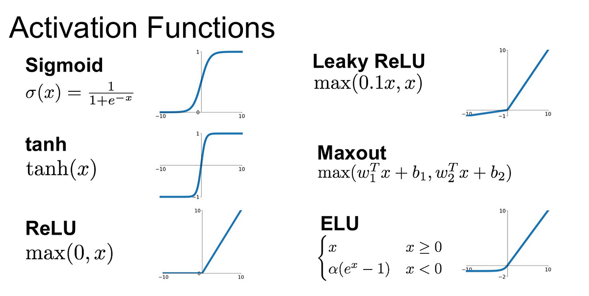
Figure 3
Finally, we should mention the initializer, which is a notion often associated with the activation functions. An initializer is a method for initializing the weights of a NN. Its goal is to avoid different nodes learning identical mappings (like Eq. (4)) within the network. This is achieved by taking the initial weights \(w_{ij}\) as random numbers from a uniform interval \([-w,+w]\) or from a gaussian distribution with mean value 0 and standard deviation \(\sigma\). One of the most famous initializers is the Glorot method, which draws samples from a uniform distribution with limits determined by the number of input and output units in the layer. The He Normal initializer is similar to the Glorot method while being specifically designed for ReLU activation function.
Number of epochs, batch size
An epoch, as referred to in the subsection "Learning/Training of a NN" is simply an iteration where the full forward- & backward propagation take place, going through all training events once. The batch size \(b\) is the number of events taken to update the weights. If \(N\) is the number of events to be trained upon, then in 1 epoch, there are \(N/b\) updates of the weights. Frequently, batch sizes are chosen as \(2^m\). The update through several batches allows multiple parameter updates per epoch. Furthermore, in the case where the partial derivative of Eq. (6) is evaluated as expectation value over a limited number of events as in the batches, the partial derivative can have a larger variance, thus sometimes helping to escape from local minima.
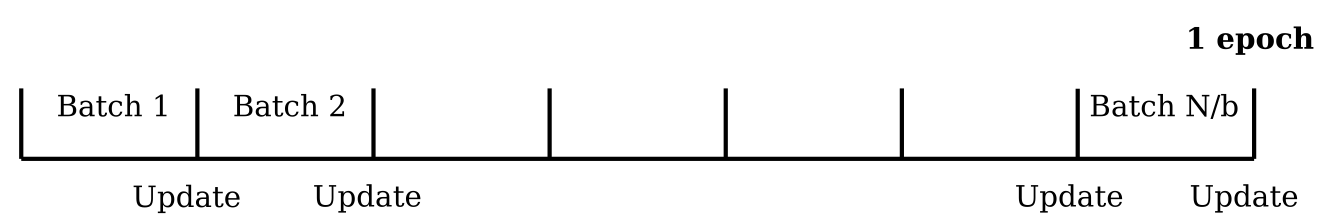
Figure 4
Advice & Possible pitfalls: It is generally a good practice to make b large as to include enough statistics for the training within an update. This can contribute to have a training/validation curve which is more stable, ie. with less fluctuations. On the other hand, if \(b\) is so large as to match the size of the training sample \(N\), there will be only one update in the training, as all data will be used to train the NN at once: this can be time consuming, and quite inefficient.
Code snippets
We should first define the basic parameters of the NN: learning- & decay-rate, architecture, and important functions (activation and initialization). In the same shot, we can also set the number of epochs and the size of the batches. NB: please note that in Keras 3 decay has changed to learning rate schedules.
activ = "relu"
LearningRate = 1.e-5
DecayRate = 1.e-2
NodeLayer = "50 50"
architecture=NodeLayer.split()
ini = "he_normal"
n_epochs = 2000
batch_size = 10000
We can then pass these parameters to the optimizer, meanwhile defining other parameters of the NN such as the number of epochs and batch size. Please note that we will cover the two latter notions in the next section. Model's compilation arguments, training parameters and optimizer:
trainParams = {'epochs': n_epochs, 'batch_size': batch_size, 'verbose': verbose}
compileArgs = {'loss': 'binary_crossentropy', 'optimizer': 'adam', 'metrics': ["accuracy"]}
myOpt = Adam(learning_rate=LearningRate, decay=DecayRate)
compileArgs['optimizer'] = myOpt
Finally, we build the model, also compiling the arguments provided above. In the example below, we first build the first layer where there are 12 input variables, then the hidden layers which have as many layers/nodes as specified in the argument \(architecture\). For both initial and hidden layers, we use ReLU as activation function and he normal as initializer. We finally define the output layer with 1 single node with a sigmoid activation function.
model = Sequential()
# 1st hidden layer: it has as many nodes as provided by architecture[0]
model.add(Dense(int(architecture[0]), input_dim=12, activation=activ, kernel_initializer=ini))
i=1
while i < len(architecture):
    model.add(Dense(int(architecture[i]), activation=activ, kernel_initializer=ini))
    i=i+1
model.add(Dense(1, activation='sigmoid')) # Output layer: 1 node, with sigmoid
model.compile(**compileArgs)
model.summary()
Once the model is defined, we train the model:
history = model.fit(xTrn, yTrn, validation_data=(xVal,yVal,weightVal), sample_weight=weightTrn, shuffle=True, callbacks=[checkpoint], **trainParams)
When defining the model as we did above, we provided the criterion for saving the best epoch as the one where the weights are such that the validation loss is at its minimum. The method below (called \(checkpoint\)), which uses the \(callbacks\) function, saves such weights, and the it is used in the line above for training:
checkpoint = callbacks.ModelCheckpoint(
    filepath=filepath+"best_weights.h5",
    verbose=1,
    save_weights_only=True,
    monitor="val_loss",
    mode="min",
    save_best_only=True
)
Sample treatment
A NN is a numerical machine, and numbers that it grinds need to be controlled, often balanced. In this section, we will cover the most common aspects of sample treatment for a NN. Apart from the first which deals with the splitting of the samples, all other subsections can be considered as data pre-processing.
Splitting: training, validation, and testing samples
We need 3 samples: one to train the NN, another to validate the training, and another where we run the analysis and get results. The main purpose of the validation sample is to see how well the NN classifies the same type of events as either S or B, this, once exposed to events which were not included in the training; we will cover more this aspect below. Therefore, the training and validation samples should be exactly similar: the fraction of the total number of events that they each represent, the composition of the samples, etc. For example: (1) If the training is performed over 25% of the signal sample, then the validation sample has to include a different still 25% of the signal sample as well; the same for the background sample. (2) If the background sample is made of 75% of Wjets and 25% of ttbar events for training, one needs to keep the same percentages for the background validation sample.
Event normalization
In the case where the values of the input variables vary by several orders of magnitude and/or are different for the various input variables, the adjusting of the NN parameters might be difficult, typically because the same weights will have to cover the possibly wildly different values. It is therefore better to render these values comparable, while they should naturally retain their discriminating power.
- One possibility is to decrease the order of magnitude of an input variable \(x_i\) while taking into account its mean value \(<x_i>\) and standard deviation \(\sigma_i\): \(x'_i = \frac{(x_i - <x_i>)}{\sigma_i}\).
- Another possibility is to normalize the input variables to the \([-1,+1]\) interval. This has the property of being simple, zero-centered (which can be interesting in some cases), and will be illustrated in among the snippets below.
Shuffling, seeding
It is important to randomly mix, ie. shuffle, S and B events in a given (training and/or validation) sample. This allows to not expose the training first or last to an event of a specific kind, which would bias the training. Having a data sample with eg. S events which come first can easily be the case when putting together, ie. concatenating, S and B events in a given (training or validation) sample.
The seeding of a NN is random if left unspecified. The specification of the seeding can be useful in the case one needs an exact reproduction of results.
Event weighting & balancing
Each event i in the training should be weighted by appropriate weight wi which reflects some physics aspect(s) and the sample specificity. Namely:
- B weights should be like : \(w_i(B) = \frac{\sigma}{N_{tot}} \times \Pi_i SF(i) \times w(i)\), where \(\sigma\) is the cross-section of the event under consideration, \(SF(i)\) is the scale factor, and \(N_{tot}\) is the total number of events. This is because the NN has to:
- Be exposed to processes proportionally to their production rate \(\sigma\) in SM. It has to be noted that the cross section \(\sigma\) has to be taken into account when the B sample includes various background processes; in the case of a single background process per sample, this can be omitted and be taken as 1.
- "Be free" of number of generated events per sample.
- Be trained with simulated events resembling as much as possible to a Data event via the appropriate scale factor(s).
- S weights should be like: \(w_i(S) = \frac{1}{N_{tot}} \times \Pi_i SF(i) \times w(i)\).
Now these S & B weights, given their definition, can be very different and lead to numerical problems in the training of the NN: for example, the validation loss can reach O(\(10^{-6,-7}\)) very early on, and lead to weird behaviors and/or under-performance. We should therefore put events on equal footing by properly balancing each event for the training. In the case of binary classification, we should have something like:
- B weights should be: \(w_i(B) \times (\frac{N_{evt}(B)}{\Sigma_i w_i(B)})\).
- S weights should be: \(w_i(S) \times (\frac{N_{evt}(B)}{\Sigma_i w_i(S)})\).
Here, both B and S weights contain the same total number of eg. B events \(N_{evt}(B)\) as to render the respective weights numerically comparable, while naturally preserving their event-by-event differences through \(w_i(B,S)\).
Code snippets
Event normalization
For normalizing the values of the input variables to the \([-1,+1]\) interval, we can do the following in a loop over the full, eg. training sample:
top = np.max(full_train[:, var]) # checks all lines by value of (variable in) column var
bot = np.min(full_train[:, var])
full_train[:, var] = (2*full_train[:, var] - top - bot)/(top - bot)
Event shuffling
For shuffling events, we can apply the following numpy command on the full eg. training sample:
np.random.shuffle(full_train)
Without the former line, the NN would be first exposed to S for many events, this because we have concatenated the entire training sample with this rather common command:
full_train = np.concatenate((train_sig, train_bkg))
To make sure, and with only the risk of redundancy, we can include the shuffle command in the very line which takes care of the training of the NN:
history = model.fit(xTrn, yTrn, validation_data=(xVal,yVal,weightVal), sample_weight=weightTrn, shuffle=True, callbacks=[checkpoint], **trainParams)
Event balancing
For balancing the events, we normalize the weights of S and B training sample as mentioned earlier. In the case of a binary classification, we can simply have:
train_bkg[:,-2] *=  train_bkg.shape[0] / np.sum(train_bkg[:,-2])
train_sig[:,-2] *=  train_bkg.shape[0] / np.sum(train_sig[:,-2])
where the weight of each data sample is the penultimate element of datasets train_bkg and train_sig, hence the \([:-2]\) numpy notation.
Metrics
Various metrics exist in order to quantify the performance, and check the sanity of a NN. Below are the main ones.
Training & Validation losses versus epoch
The training of the NN by definition minimizes the loss, so this latter should decrease versus the epochs for events used for training. So the calculated loss in the validation sample where the weights, as calculated for a given epoch, should have the effect of decreasing the loss in a sample non-exposed to the training. However, a training is never perfect and the loss will never reach nil. As a result, and after a number of epochs, the losses will reach and remain at a minimal and non-zero value. A typical good and realistic example of how training and validation losses should be is given in the plot below: both training and validation losses decrease and plateau after a while, and the validation loss is superior or equal to the training loss, as we do not expect the same weights to yield a better result in the validation sample than for the training sample itself.

Figure 5
The following situations are cases where one should pay attention or pitfalls:
- The training & validation losses are increasing after having reached a minimum. This can happen when, ie. from an epoch, the NN is over-fitting the data. In such a case, collecting the weights of the NN at the end of the training will not be optimal, as they will correspond to a case where the loss function isn't minimal, resulting in an under-performing NN. In such a case, as illustrated above, one can/should collect the weights of the epoch where the validation loss is at its minimum.
- Validation loss smaller than training loss. There can be 3 reasons why this can happen.
- Regularization is applied during training, but not during validation. Regularization leads to a set of weights which generalize better, ie NN results which are more stable for different samples, but also to slightly lower classification performance (eg. higher loss, lower accuracy).
- Depending on the software used, the training loss can be calculated at the end of each batch and then averaged over all batches of a given epoch, while the validation loss after a full epoch. In such a case, the validation loss is calculated over the full validation set (all batches), without updating at the end of each batch. For example, the default option in Keras is to return the training loss as averaged over the individual batch losses.
- The validation can be easier (to learn) than the training sample. This can happen if the validation and training sample are not formed from the same dataset, or if, for any reason, the validation data isn't as hard to classify as the training data. This can also happen if some training events are also mixed in the validation sample. If the code creating the training, validation and testing samples splits them correctly, from the same dataset, these shouldn't happen.
True/False positive/negative
In a binary classification, each event is either in one or the other class, classes that we call "positive" and "negative" (eg. S or B). And each event is predicted to be in one of these two classes by the NN. We can define a confusion matrix which gives the fraction of each true category as classified in a predicted class, see the figure below. Obviously, the more diagonal is this matrix, the better is the classification of the NN; we will cover a quantitative measure of the entire matrix in the subsequent section.
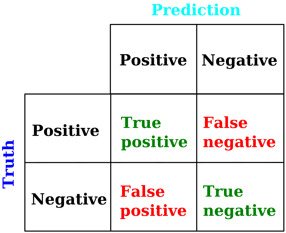
Figure 6
A criterion for a good classifier can be to maximize the fraction of true positive events (ie. S events classified as S) while also minimizing the false positive (ie. B events classified as S). We can report the rate of each of these events for various cuts on the NN output, as illustrated in the figure below. With this criterion, the classification power of the NN is optimal when the curve the peaks as much as possible to the top-left corner of this plot (green curve). In the opposite case, when the classifier produces as much true positive as false positive, it means that it does not have any classification power (red curve). A classifier whose curve lies between these limits is fine, but again, the closer it gets to the top-left corner, the better.
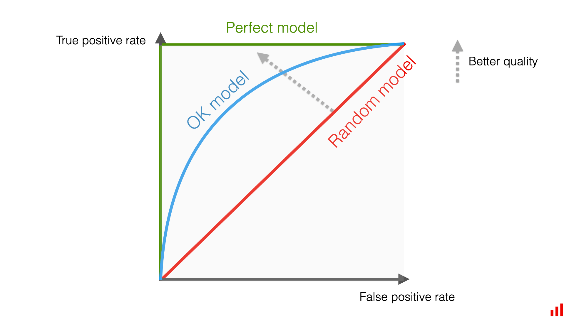
Figure 7
A quantitative measure of this "peaking" by the area under the (roc) curve, is reported in the figure below: the greater is this area, the better is the classification.

Figure 8
Accuracy versus epoch
A quantity measuring in a single shot all the elements of the binary confusion matrix is the accuracy, defined as the ratio of events classified in their correct classes to all events:
In the example below, we can observe an NN improving the accuracy after each epoch, and somehow plateau after a certain number of epochs:
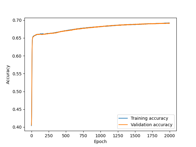
Figure 9
Multi-class NN: confusion matrix
In the case of a multi-class NN, the confusion simply has more than two classes, as illustrated below. Again, the more diagonal is the matrix, the more correct is the classification.
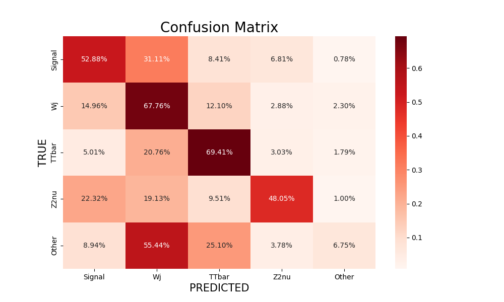
Figure 10
Over-training
We briefly mentioned at the start of the previous section the justification for having a validation sample. Through a comparison of the performance of the NN in the training and validation samples, one is testing the reproducibility of the NN: whether the NN 's response is similar for events that it has been trained upon (training sample) or events that it hasn't been exposed to (validation sample); this response should not depend on events. Therefore, the NN's response should be similar in the training and validation samples, for both S and B events.
\rightarrow One simple way to check for over-training is to overlay the NN output distribution in the training and validation samples (for S events on one hand, and for B events on the other), and make sure that that they are compatible within statistical uncertainties. In the example below, a comparison is provided between the validation and test samples.
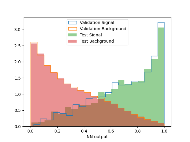
Figure 11
Assess performance of classification in analysis
An area under the receiver operating characteristics curve (auroc) is essentially measuring true S and B events being predicted as S events. Maximizing the auroc is mainly maximizing the S/B ratio. Here, there is no uncertainty of any kind taken into account. This is obviously insufficient for gauging the classification power of an ML tool in a real analysis situation, where both statistical and systematic uncertainties have to be accounted for. Beyond the auroc's, and in order to capture a more complete statistical picture of an analysis, one can define a Figure Of Merit, which is a quantity :
where S and σT are the signal yield and the total uncertainty, respectively. The total uncertainty is the quadratic sum of the systematic uncertainty on the background σB and the total statistical uncertainty, itself the quadratic sum of the statistical uncertainties on the signal and background. If we assume Poisson uncertainty for the statistical uncertainty on the yields, we have:
where B is the background yield. If the analyzer knows that the measurement is going to be dominated by statistical uncertainties, then the expression above simplifies to:
If the analyzer further thinks that the statistical uncertainty on the signal is negligible when compared to the one on the background, the expression further simplifies to the well known expression:
It has to be noted that even with the most simplifying assumptions, the FOM above is close to, but not the same than S/B, which is effectively what the auroc is about.
Code snippets
Loss & accuracy curves
For obtaining the loss and accuracy (versus epoch) curves, we should first include them among the very list of arguments to be compiled. For the loss, we should specify which type of loss we want, and for the accuracy, we should include it among the metrics:
compileArgs = {'loss': 'binary_crossentropy', 'optimizer': 'adam', 'metrics': ["accuracy"]}
Then, and after having trained the model, we can obtain these curves for the training and validation samples with the following lines:
loss = history.history['loss']
val_loss = history.history['val_loss']
acc = history.history["accuracy"]
val_acc = history.history['val_accuracy']
ROC curves
In order calculate the roc curve and the auroc, one should first import the corresponding libraries:
from sklearn.metrics import roc_curve, auc
We can then obtain the roc cruve and the auroc, for both the training and validation samples, with the following lines:
y_pred_Trn = model.predict(xTrn).ravel()
fpr_Trn, tpr_Trn, thresholds_Trn = roc_curve(yTrn, y_pred_Trn)
auc_Trn = auc(fpr_Trn, tpr_Trn)
y_pred_Val = model.predict(xVal).ravel()
fpr_Val, tpr_Val, thresholds_Val = roc_curve(yVal, y_pred_Val)
auc_Val = auc(fpr_Val, tpr_Val)
Full codes
The purpose of this part is to give an example of full and working script, for each type of classification (binary and multi-class). These scripts are meant to be illustrative and are naturally improvable. They are commented quite extensively as to guide explain the different aspects of the code. Each code has two type of outputs:
- Plots which provide information about the training (eg. loss, accuracy versus epoch)
- Files which are usable for further investigation of the NN (eg. performance).
Both scripts are based on python, and use Keras. Both run on csv files where each line represents the entries for an event, and where:
- the N first columns are the N input variables: discriminating features, which can either be continuous or discrete variables. Examples: \(p_T\) and spatial distribution of various reconstructed particles, invariant masses, charge and identification and isolation variables of leptons, jet- and b-tag multiplicities, b-tagging discriminant distributions, ...
- followed by a column containing the event weight:
- and then by a column containing the string specifying the physical process of the event; the way that the script expects this string is in the NameProcess.root (eg. ttbar.root) form.
This order is important as the numpy manipulation the various elements of the csv file in the script naturally takes it into account. In a certain measure, and for secondary aspects, the two codes have different functionalities, as to illustrate various possible outcomes.
Binary
The script for the binary NN uses numpy for the manipulation of vectors. It is meant to turn on csv files which provide N=12 input variables. It is integrating all snippets mentioned in previous sections. Its outcomes are:
- 3 plots: TrnVal_loss.png, TrnVal_accuracy.png, TrnVal_roc.png, respectively showing the evolution of the loss, accuracy, and roc curves as a function of the epoch, these for the training and validation samples.
- A file for weights: best_weights.h5 which has the weights of the NN corresponding to the epoch where the validation loss is the lowest, ie. the best weights one can get from the NN training. This file is useful downstream calculations (eg. for calculating the performance of the NN).
- 2 files val_output.csv and test_output.csv, where the outputs of the NN are saved for the validation and test samples, and which are necessary for downstream calculations.
Full Code Binary
import os
os.environ['TF_CPP_MIN_LOG_LEVEL']='2'
from tensorflow.python.keras import *
from tensorflow.python.keras.optimizer_v2.adam import Adam
from tensorflow.python.keras.models import Sequential
from tensorflow.python.keras.layers import Dense, Dropout, AlphaDropout
from tensorflow.python.keras.regularizers import l2
from tensorflow.keras.mixed_precision import experimental as mixed_precision

#from tensorflow.python.keras.utils import metrics_utils

import numpy
import time
import pandas
from sklearn.metrics import confusion_matrix, cohen_kappa_score, roc_curve, auc
import matplotlib.pyplot as plt
import pickle
import numpy as np
import pandas as pd

def assure_path_exists(path):
    if not os.path.exists(path):
        os.mkdir(path)

def load_data(path, tag):
    """ Read data from CSV
    Args:
    path (str): path to the data
    tag (int): 1 if signal, 0 if background
    Returns:
    np.c_[data, tag] (np.array): array with data and tag
    label (np.array): array with the name of event process
    """
    full_data = np.loadtxt(path, delimiter=",", dtype="str")
    tag = np.ones(len(full_data))*tag
    label = full_data[:, -1]
    data = np.array(full_data[:,:-1], dtype="float")
    return np.c_[data, tag], label

def mae(y_true, y_pred):
    n = len(y_true)
    error = np.abs(y_true - y_pred)
    return error / n

if __name__ == "__main__":
    import argparse
    import sys

    # Uses the "weight" variable of roottuples: provided as (N(input vars)+1)th variable in csv files
    # Passed on weightTrn & weightVal for appropriate samples
    # Weighting each event by these vectors: effectively weighting samples of various XS & Nevts, thus
    # no need of a single "Background.root"

    # Input arguments from command line
    parser = argparse.ArgumentParser(description='Process the command line options')
    parser.add_argument('-v', '--verbose', action='store_true', help='Whether to print verbose output')
    parser.add_argument('-y', '--year', type=str, required=True, help='Year of data being trained')
    parser.add_argument('-c', '--channel', type=str, required=True, help='Final state of data being trained')
    parser.add_argument('-n', '--name', type=str, required=True, help='model name')

    args = parser.parse_args()

    ### Read input arguments
    year = args.year
    channel=args.channel
    name=args.name
    verbose = 0
    if args.verbose:
        verbose = 1
    ###

    ### NN parameters
    activ = "relu"
    learning_rate = 5.e-3
    decay_rate = 0.
    # Each number (here 50) is the number of nodes (Nnode) in each layer.
    # The number of different Nnode (here 2) is the number of layers.
    NodeLayer = "50 50"
    architecture=NodeLayer.split()
    ini = "he_normal" # Function for initialising the random weights of the layer
    n_epochs = 2000
    batch_size = 5000
    dropout_rate = 0.
    ###

    # Model's compilation arguments, training parameters and optimizer
    compileArgs = {'loss': 'binary_crossentropy', 'optimizer': 'adam', 'metrics': ["accuracy"]}
    trainParams = {'epochs': n_epochs, 'batch_size': batch_size, 'verbose': verbose}
    print(Adam)
    # Define optimizer which has the learning- & decay-rates
    myOpt = Adam(lr=learning_rate, decay=decay_rate)
    # Protect from rounding errors: Number by which the loss-function is multiplied to protect from rounding errors
    #                               dynamically scales the loss to prevent underflow
#    myOpt = mixed_precision.LossScaleOptimizer(myOpt, 1e5)
    compileArgs['optimizer'] = myOpt

    # Creating the directory where the files will be stored
    dirname = year+"_"+channel+"_"+name
    filepath = "models/{}/".format(dirname)
    if not os.path.exists(filepath):
        os.mkdir(filepath)

    # Printing info and starting time
    if args.verbose:
        print("Dir "+filepath+" created.")
        print("Starting the training")
        start = time.time()

    ##### Build the model
    model = Sequential()

    # 1st hidden layer: it has as many nodes as provided by architecture[0]: 12 b/c that much input variables
    model.add(Dense(int(architecture[0]), input_dim=12, activation=activ, kernel_initializer=ini))

    i=1
    while i < len(architecture) :
        model.add(Dense(int(architecture[i]), activation=activ, kernel_initializer=ini))
#        model.add(kernel_regularizer=l2(1e-5))
#        model.add(Dropout(dropout_rate))
        i=i+1
    model.add(Dense(1, activation='sigmoid')) # Output layer: 1 node, with sigmoid

    model.compile(**compileArgs)
    model.summary()
    #####

    # Read input data
    print("LOADING DATA")
    # Do the labeling for S & B to 1 & 0 for train, val and test samples
    # For train sample: avoid writing the value of label with "_",
    train_sig, _ = load_data("data/train_sig.csv", 1)
    train_bkg, _ = load_data("data/train_bkg.csv", 0)
    # validation sample
    val_sig, label_val_sig = load_data("data/val_sig.csv", 1)
    val_bkg, label_val_bkg = load_data("data/val_bkg.csv", 0)
    val_label = np.concatenate((label_val_sig, label_val_bkg))
    val_label = np.array([l[:-5] for l in val_label]) # Keep all file/process name except ".root" to identify processes
    # test sample
    test_sig, label_test_sig = load_data("data/test_sig.csv", 1)
    test_bkg, label_test_bkg = load_data("data/test_bkg.csv", 0)
    test_label = np.concatenate((label_test_sig, label_test_bkg))
    test_label = np.array([l[:-5] for l in test_label]) #  Keep all file/process name except ".root" to identify processes
    # Concatenation of variables and weights only
    # NB: could have been done in the general form (concatenate the total object, as above)
    test_data = np.concatenate((test_sig[:, :-2], test_bkg[:, :-2]))
    test_weight = np.concatenate((test_sig[:, -2], test_bkg[:, -2]))

    # Weight normalisation, event balancing:
    # Render the sum of S events equal to sum of B events
    # The totality of weights should be equal, even though the relative weights
    # among B or S signal are correct by weighting each event by the "weight"
    # variable in the roottuples
#    train_sig[:, -2]*=np.sum(train_bkg[:, -2])/np.sum(train_sig[:, -2])
    # AND
    # each sample should be numerically not too small: normalize by the N(B),
    # both for S & B, in both training & validation sample
    train_bkg[:,-2] *=  train_bkg.shape[0] / np.sum(train_bkg[:,-2])
    train_sig[:,-2] *=  train_bkg.shape[0] / np.sum(train_sig[:,-2])
    # Save unweighted values of validation weights, to be written in val_output.csv
    full_val_not_scaled = np.concatenate((val_sig, val_bkg))
    weightVal_not_scaled = full_val_not_scaled[:, -2]
    val_bkg[:,-2] *=  val_bkg.shape[0] / np.sum(val_bkg[:,-2])
    val_sig[:,-2] *=  val_bkg.shape[0] / np.sum(val_sig[:,-2])

    # Concatenate signal and background for train and validation
    full_train = np.concatenate((train_sig, train_bkg))
    full_val = np.concatenate((val_sig, val_bkg))

    # Variables normalisation to [-1,+1]
    # Looping over number of variables:
    #   shape = Dimension of the full_train (variables * Nevts) array
    #   shape[0] gives lines: the dimension is Nevts
    #   shape[1] gives columns: the dimension here is 12 (for input vars.) + 1 (weight) + 1 (tag=0,1)
    for var in range(full_train.shape[1] - 2):
    top = np.max(full_train[:, var]) # checks all lines by value of (variable in) column var
    bot = np.min(full_train[:, var])
    full_train[:, var] = (2*full_train[:, var] - top - bot)/(top - bot)
    full_val[:, var] = (2*full_val[:, var] - top - bot)/(top - bot)
    test_data[:, var] = (2*test_data[:, var] - top - bot)/(top - bot)

    np.random.shuffle(full_train) # Without this line: NN first exposed to S for many events: b/c fullt_train = np.concatenate((train_sig, train_bkg))
    xTrn = full_train[:, :-2] # Input of NN (kinematic variables)
    yTrn = full_train[:, -1] # Target of NN (1 for signal, 0 for background)
    weightTrn = full_train[:, -2]
    xVal = full_val[:, :-2]
    yVal = full_val[:, -1]
    weightVal = full_val[:, -2]

    # Define criterium for best epoch saving
    # Returns the weights as they are at the minimum, b/c of argument of mode
    checkpoint = callbacks.ModelCheckpoint(
    filepath=filepath+"best_weights.h5",
    verbose=1,
    save_weights_only=True,
    monitor="val_loss",
    mode="min",
    save_best_only=True)

    ### Train model ###
    history = model.fit(xTrn, yTrn, validation_data=(xVal,yVal,weightVal), sample_weight=weightTrn,shuffle=True, callbacks=[checkpoint], **trainParams)

    loss = history.history['loss']
    val_loss = history.history['val_loss']
    acc = history.history["accuracy"]
    val_acc = history.history['val_accuracy']

    # Saving accuracy and loss values in a pickle file for later plotting
    pickle.dump(acc, open(filepath+"acc.pickle", "wb"))
    pickle.dump(loss, open(filepath+"loss.pickle", "wb"))
    pickle.dump(val_acc, open(filepath+"val_acc.pickle", "wb"))
    pickle.dump(val_loss, open(filepath+"val_loss.pickle", "wb"))

    # Getting the roc curve
    y_pred_Trn = model.predict(xTrn).ravel()
    fpr_Trn, tpr_Trn, thresholds_Trn = roc_curve(yTrn, y_pred_Trn)
    auc_Trn = auc(fpr_Trn, tpr_Trn)
    y_pred_Val = model.predict(xVal).ravel()
    fpr_Val, tpr_Val, thresholds_Val = roc_curve(yVal, y_pred_Val)
    auc_Val = auc(fpr_Val, tpr_Val)

    # Getting errors
#    mae_Trn = mae(yTrn, y_pred_Trn)
#    mae_Val = mae(yVal, y_pred_Val)

    # Plot loss curves
    plt.figure(1)
    plt.plot(loss, label="Training loss")
    plt.plot(val_loss, label="Validation loss")
    plt.legend()
    plt.xlabel('Epoch')
    plt.ylabel('Loss')
#    plt.yscale("log")
    plt.savefig(filepath+"TrnVal_loss.png")
    # Plot accuracy curves
    plt.figure(2)
    plt.plot(acc, label="Training accuracy")
    plt.plot(val_acc, label="Validation accuracy")
    plt.legend()
    plt.xlabel('Epoch')
    plt.ylabel('Accuracy')
#    plt.yscale("log")
    plt.savefig(filepath+"TrnVal_accuracy.png")
    # Plot ROC curves
    plt.figure(3)
    plt.plot([0, 1], [0, 1], 'k--')
    plt.plot(fpr_Trn, tpr_Trn, label='Training ROC (area = {:.2f})'.format(auc_Trn))
    plt.plot(fpr_Val, tpr_Val, label='Validation ROC (area = {:.2f})'.format(auc_Val))
    plt.legend()
    plt.xlabel('False positive rate')
    plt.ylabel('True positive rate')
    plt.savefig(filepath+"TrnVal_roc.png")
#    plt.figure(4)
##    plt.plot([0, 100], 'k--')
#    plt.plot(mae_Trn, label="Training MAE")
#    plt.plot(mae_Val, label="Validation MAE")
#    plt.legend()
#    plt.xlabel('N(events)')
#    plt.ylabel('MAE')
#    plt.savefig(filepath+"TrnVal_mae.png")

    # Time of the training
    if args.verbose:
        print("Training took ", (time.time()-start)//60, " minutes")

    # Getting predictions
    if args.verbose:
        print("Getting predictions")

    model.load_weights(filepath + "best_weights.h5") # Loading best epoch weights

    # Compute and save prediction for best epoch
    trnPredict = model.predict(xTrn)
    valPredict = model.predict(xVal)
    testPredict = model.predict(test_data)
#    np.savetxt(filepath+"val_output.csv", np.c_[valPredict, weightVal, val_label], delimiter=",", fmt="%s")
    np.savetxt(filepath+"val_output.csv", np.c_[valPredict, weightVal_not_scaled, val_label], delimiter=",", fmt="%s")
    np.savetxt(filepath+"test_output.csv", np.c_[testPredict, test_weight, test_label], delimiter=",", fmt="%s")

    # Outputs
#    plt.savefig(filepath+"loss.png")
    val_file = open(filepath + "val_loss.pickle", "rb")
    val = pickle.load(val_file)
    print("Epoch of the best training: ",np.argmin(val))
Multiclass
The script for the multi-class NN is classifying 5 different processes (Signal, Wjets, TTbar, Z2nu, Other), and has thus 5 different classes. It uses panda for the manipulation of vectors, and is performing this manipulation slightly differently than in the binary script, but with similar outcomes. It is meant to turn on csv files which provide N=17 input variables. This script is performing 2 loops, the first being nested in the second:
- It is simply running 10 times, letting all random-based processes (initialization, shuffling, seeding) produce 10 different results, which are close in performance.
- It is scanning the decay-rate from \(10^{-5}\) to \(10^{-3}\).
It goes without saying that these loops can be taken out, or modified. This script has performance calculation capacity embedded in it, and doesn't need a downstream script to be run. The outcomes of the script are:
- A file 17var_fom.csv necessary for possible downstream performance calculations.
- 10 different subdirectories, corresponding to the 10 runs, with each containing:
- 2 plots: TrnVal_loss.png, TrnVal_accuracy.png, as in the binary case.
- A file for weights best_weights.h5, as in the binary case.
- A subdirectory FOM_figures_runs/ which has the performance plots of all 10 runs in it.
As for the event balancing used in the case of multi-class NN, we do an event weighting similar yet different than in the "Event weighting & balancing" section. Interested users are invited to look at slides 10-13 and 23 of this presentation; referring to these slides, the balancing scheme used in this script is the "SQRT".
Full Code Multiclass
import os
os.environ['TF_CPP_MIN_LOG_LEVEL']='2'
from tensorflow.python.keras import *
from tensorflow.python.keras import backend as K
from tensorflow.python.keras.optimizer_v2.adam import Adam
from tensorflow.python.keras.models import Sequential
from tensorflow.python.keras.layers import Dense, Dropout
from tensorflow.python.keras.regularizers import l2
#from tensorflow.keras.mixed_precision import experimental as mixed_precision

import tensorflow as tf

import numpy
import time
import pandas as pd
from sklearn.metrics import confusion_matrix, cohen_kappa_score, roc_curve, auc
import seaborn as sns
import matplotlib.pyplot as plt
import pickle
import numpy as np
import pandas as pd

def assure_path_exists(path):
    if not os.path.exists(path):
        os.mkdir(path)

# Takes strings of processes from XYZ.root and returns abbreviated name XY as name of the process
def rename_rows(label):
    filenames = set(label)
    names = []
    for i in filenames:
        tag = i[0] + i[1]
        if tag=="Wj":
            names += [i, "Wjets"]
        elif tag=="TT":
            names += [i, "TTbar"]
        elif tag=="ZJ":
            names += [i, "Z2nu"]
        else:
            names += [i, "Other"]
    N = len(names)
    dictionary = {names[i] : names[i+1] for i in range(0,N,2)}
    return dictionary


# Maps a 1 for a specific process and 0's elsewhere, in an array of (here 5) elements
def Tag(dataframe):
    data = dataframe.copy() # Makes a copy -> another address in memory
    # Mapping (input mapping) of various process strings to 1, and 0's for other processes
    data["SigTag"] = data.index.map({"Signal":1}).fillna(0)
    data["WjTag"] = data.index.map({"Wjets":1}).fillna(0)
    data["TTTag"] = data.index.map({"TTbar":1}).fillna(0)
    data["Z2nuTag"] = data.index.map({"Z2nu":1}).fillna(0)
    data["OtherTag"] = data.index.map({"Other":1}).fillna(0)
    # Makes the arry of (here 5) elements made of 0/1
    return pd.concat([data["SigTag"],data["WjTag"],data["TTTag"],data["Z2nuTag"], data["OtherTag"]], axis=1)

N_runs=10

print("Loading data...")

# PREPARING DATA #######################################

### Reading data
names = ["LepChg", "LepPt", "LepEta", "Dxy", "Dz", "RelIso", "Met", "mt", "Njet",
        "Jet1Pt", "Jet2Pt", "HT", "NbLoose", "JetHBpt", "JetHBCSV", "JetB2pt", "DrJetHBLep", "Weights", "Tag"]

# index_col defines last column as index (row names) of DataFrame. Resulting DataFrame has xyz.root as its last column (indexing starts @ 0)
# When interpreting it as index column it plays the same part as do numbers 0,1,2,3... in numpy array (eg. a[i] is i-th element of array a).
# It disappears from the list of values you are "interpreting as data"
train_sig = pd.read_csv("17var/data/train_sig.csv", header=None, names=names, index_col=18)
train_bkg= pd.read_csv("17var/data/train_bkg.csv", header=None, names=names, index_col=18)

val_sig = pd.read_csv("17var/data/val_sig.csv", header=None, names=names, index_col=18)
val_bkg = pd.read_csv("17var/data/val_bkg.csv", header=None, names=names, index_col=18)

test_sig = pd.read_csv("17var/data/test_sig.csv", header=None, names=names, index_col=18)
test_bkg = pd.read_csv("17var/data/test_bkg.csv", header=None, names=names, index_col=18)

### Get S=(550,520) lines
val_sig_S = val_sig.loc['T2DegStop_550_520.root'] # Filter DataFrame rows (only 1 argument) by name
val_sig_S.index = ['Signal'] * len(val_sig_S)

train_sig_S = train_sig.loc['T2DegStop_550_520.root']
train_sig_S.index = ['Signal'] * len(train_sig_S)

### Index = category of the process ("Signal", "Wjets", "TTbar", "Z2nu", "Other")
train_sig.index = ['Signal'] * len(train_sig) #
names = rename_rows(train_bkg.index) # train_bkg.index holds the name of the process from index_col=18
train_bkg = train_bkg.rename(index=names) # Rename (here) index labels

val_sig.index = ['Signal'] * len(val_sig)
names = rename_rows(val_bkg.index)
val_bkg = val_bkg.rename(index=names)

test_sig.index = ['Signal'] * len(test_sig)
names = rename_rows(test_bkg.index)
test_bkg = test_bkg.rename(index=names)

### Separate processes
train_wj = train_bkg.loc[["Wjets"]]
train_tt = train_bkg.loc[["TTbar"]]
train_z2nu = train_bkg.loc[["Z2nu"]]
train_other = train_bkg.loc[["Other"]]

val_wj = val_bkg.loc[["Wjets"]]
val_tt = val_bkg.loc[["TTbar"]]
val_z2nu = val_bkg.loc[["Z2nu"]]
val_other = val_bkg.loc[["Other"]]

for dlta in range(0,1): # ?

    ### Weight normalisation

    delta = dlta # Useless

    N_sig = train_sig.shape[0]

    S = train_sig["Weights"].sum()
    W = train_wj["Weights"].sum()
    T = train_tt["Weights"].sum()
    Z = train_z2nu["Weights"].sum()
    O = train_other["Weights"].sum()

    sig = 1.
    wj = np.sqrt(W/S)
    tt = np.sqrt(T/S)
    z2nu = np.sqrt(Z/S)
    other = np.sqrt(O/S)

    weightTrn_sig = train_sig["Weights"]*N_sig/S*sig
    weightTrn_wj = train_wj["Weights"]*N_sig/W*wj
    weightTrn_tt = train_tt["Weights"]*N_sig/T*tt
    weightTrn_z2nu = train_z2nu["Weights"]*N_sig/Z*z2nu
    weightTrn_other = train_other["Weights"]*N_sig/O*other

    N_sig = val_sig.shape[0]

    S = val_sig["Weights"].sum()
    W = val_wj["Weights"].sum()
    T = val_tt["Weights"].sum()
    Z = val_z2nu["Weights"].sum()
    O = val_other["Weights"].sum()

    sig = 1.
    wj = np.sqrt(W/S)
    tt = np.sqrt(T/S)
    z2nu = np.sqrt(Z/S)
    other = np.sqrt(O/S)

    weightVal_sig = val_sig["Weights"]*N_sig/S*sig
    weightVal_wj = val_wj["Weights"]*N_sig/W*wj
    weightVal_tt = val_tt["Weights"]*N_sig/T*tt
    weightVal_z2nu = val_z2nu["Weights"]*N_sig/Z*z2nu
    weightVal_other = val_other["Weights"]*N_sig/O*other

        ###

    # Full train
    full_train = pd.concat([train_sig, train_wj, train_tt, train_z2nu, train_other])
    full_train_weights = pd.concat([weightTrn_sig, weightTrn_wj, weightTrn_tt, weightTrn_z2nu, weightTrn_other])
    weights_not_scaled_train = full_train["Weights"]
    ### Only S=(550,520) for plotting
    full_train_S = pd.concat([train_sig_S, train_wj, train_tt, train_z2nu, train_other])
    weights_not_scaled_train_S = full_train_S["Weights"]

    # Full validation
    full_val = pd.concat([val_sig, val_wj, val_tt, val_z2nu, val_other])
    full_val_weights = pd.concat([weightVal_sig, weightVal_wj, weightVal_tt, weightVal_z2nu, weightVal_other])
    weights_not_scaled_val = full_val["Weights"]
    ### Only S=(550,520) for plotting
    full_val_S = pd.concat([val_sig_S, val_wj, val_tt, val_z2nu, val_other])
    weights_not_scaled_val_S = full_val_S["Weights"]

    # Full test
    full_test = pd.concat([test_sig, test_bkg])
    full_test_weights = full_test["Weights"]
    weights_not_scaled_test = full_test["Weights"]

    ### Variable normalisation to [-1,1]
    top = full_train.max() ; bot = full_train.min()
    full_val = (2*full_val-top-bot)/(top-bot)
    full_val_S = (2*full_val_S-top-bot)/(top-bot)
    full_test = (2*full_test-top-bot)/(top-bot)
    full_train = (2*full_train-top-bot)/(top-bot)
    full_train_S = (2*full_train_S-top-bot)/(top-bot)

        # Replace original weights with balanced weights
    full_val = pd.concat([full_val.drop("Weights", axis=1), full_val_weights], axis=1) # Along columns (axis=1): drops the column "Weights" & replaces
    full_val_S = pd.concat([full_val_S.drop("Weights", axis=1), weights_not_scaled_val_S], axis=1)
    full_train_S = pd.concat([full_train_S.drop("Weights", axis=1), weights_not_scaled_train_S], axis=1)
    full_test = pd.concat([full_test.drop("Weights", axis=1), full_test_weights], axis=1)
    full_train = pd.concat([full_train.drop("Weights", axis=1), full_train_weights], axis=1)

    ### INFO for plotting
    xTrn_p = full_train.drop("Weights", axis=1)
    yTrn_p = Tag(full_train)
    weightTrn_p = weights_not_scaled_train
    ###### S=(550,520)
    xTrn_S = full_train_S.drop("Weights", axis=1)
    yTrn_S = Tag(full_train_S)
    weightTrn_S = weights_not_scaled_train_S

    xVal_p = full_val.drop("Weights", axis=1)
    yVal_p = Tag(full_val)
    weightVal_p = weights_not_scaled_val
    ###### S=(550,520)
    xVal_S = full_val_S.drop("Weights", axis=1)
    yVal_S = Tag(full_val_S)
    weightVal_S = weights_not_scaled_val_S

    xTest_p = full_test.drop("Weights", axis=1)
    yTest_p = Tag(full_test)
    weightTest_p = weights_not_scaled_test

    ### Shuffling
    full_train = full_train.sample(frac=1) # Returns a random sample of items from an axis of object
    full_val = full_val.sample(frac=1)     # with fraction of axis items to return
    full_test = full_test.sample(frac=1)

    ### NN training
        # When dropping the weights, only input vars remain, the Tag column having been interpreted as index
    xTrn = full_train.drop("Weights", axis=1)
    yTrn = Tag(full_train)
    weightTrn = full_train["Weights"]

    xVal = full_val.drop("Weights", axis=1)
    yVal = Tag(full_val)
    weightVal = full_val["Weights"]

    xTest = full_test.drop("Weights", axis=1)
    yTest = Tag(full_test)
    weightTest = full_test["Weights"]

    for q in range(3, 5):
        learning_rate = 5.e-5
        decay_rate = 10**(-1.*q)
        NodeLayer = "100 100" # Means 2 layers of 100 nodes each
        architecture=NodeLayer.split()
        ini = "he_normal" # Function for initialising the random weights of the layer
        n_epochs = 1000
        batch_size = 5000
        dropout_rate = 0.

        verbose=0

        activ = "tanh"
        loss_function = "categorical_crossentropy"

        name="levels_00"#+str(dlta)
        lrdr="LR4e-1_DR5e-7"

        dirname ="2016_1l_Tanh_CatCrossEnt_100-100_L5e-5_D1e-"+str(q)

        fom_data = pd.DataFrame(columns=["Scaling Function","NN Configuration","Activation Function", "Loss Function", "Learning Rate", "Decay Rate", "Max Val FOM", "at x_cut", "Test FOM", "Max Test FOM"])

        org_path = "17var_models_5C/"+dirname+"/"
        if not os.path.exists(org_path):
            os.mkdir(org_path)

        for k in range(N_runs):
            string = "17var_models_5C/{}/run"+str(k)+"/"
            filepath = string.format(dirname)
            if not os.path.exists(filepath):
                os.mkdir(filepath)
            # MULTICLASS NEURAL NETWORK TRAINING ###################

            # Model's compilation arguments, training parameters and optimizer #categorical_crossentropy
            compileArgs = {'loss':loss_function, 'optimizer': 'adam', 'metrics': ["accuracy"]}
            trainParams = {'epochs': n_epochs, 'batch_size': batch_size, 'verbose': verbose}
            print(Adam)
            # Define optimizer which has the learning- & decay-rates
            myOpt = Adam(lr=learning_rate, decay=decay_rate)
            compileArgs['optimizer'] = myOpt

            # Printing info and starting time
            print("Dir "+filepath+" created.")
            print("Starting the training")
            start = time.time()

            ### Build the NN model
            model = Sequential()
            # 1st hidden layer: it has as many nodes as provided by architecture[0]
            # input_dim: as many as input variables
            model.add(Dense(int(architecture[0]), input_dim=17, activation=activ, kernel_initializer=ini))
            i=1
            while i < len(architecture) :
                model.add(Dense(int(architecture[i]), activation=activ, kernel_initializer=ini))
                i=i+1
            model.add(Dense(5, activation='softmax')) # Output layer: 5 nodes, with softmax b/c multi-class NN
            #        model.add(kernel_regularizer=l2(1e-5))
            #        model.add(Dropout(dropout_rate))
            model.compile(**compileArgs)
            model.summary()
            ########
            # Define criterium for best epoch saving
            # Returns the weights as they are at the minimum, b/c of argument of mode
            checkpoint = callbacks.ModelCheckpoint(filepath=filepath+"best_weights.h5", verbose=1, save_weights_only=True, monitor="val_loss", mode="min", save_best_only=True)

            ### Train model ###
            history = model.fit(xTrn, yTrn, validation_data=(xVal,yVal,weightVal), sample_weight=weightTrn,shuffle=True,  callbacks=[checkpoint], **trainParams)
            # Get weights for best epoch
            model.load_weights(filepath + "best_weights.h5")
            ### Time of the training
            print("Training took: ", (time.time()-start)//60, " minutes")

            ########################################################


            ########################################################

            # SAVING OUTPUT ########################################

            # LOSS #################################################
            loss = history.history['loss']
            val_loss = history.history['val_loss']

            plt.figure(figsize=(10, 6))
            plt.plot(loss, label="Training loss")
            plt.plot(val_loss, label="Validation loss")
            plt.ylabel("LOSS")
            plt.xlabel("EPOCHS")
            plt.legend()

            plt.savefig(filepath+"TrnVal_loss.png")
            ########################################################

            # ACCURACY #############################################
            acc = history.history["accuracy"]
            val_acc = history.history["val_accuracy"]

            plt.figure(figsize=(10, 6))
            plt.plot(acc, label="Training accuracy")
            plt.plot(val_acc, label="Validation accuracy")
            plt.ylabel("ACCURACY")
            plt.xlabel("EPOCH")
            plt.yscale("log")
            plt.legend()

            plt.savefig(filepath+"TrnVal_accuracy.png")
            ########################################################

            ### Saving accuracy and loss values in a pickle file for later plotting
            pickle.dump(acc, open(filepath+"acc.pickle", "wb"))
            pickle.dump(loss, open(filepath+"loss.pickle", "wb"))
            pickle.dump(val_acc, open(filepath+"val_acc.pickle", "wb"))
            pickle.dump(val_loss, open(filepath+"val_loss.pickle", "wb"))

            ### Test
            predicted_test = pd.DataFrame(model.predict(xTest_p)).rename(columns={0:"Signal",1:"Wjets",2:"TTbar",3:"Z2nu",4:"Other"})
            true_test = yTest_p

            predicted_test["Predicted"] = predicted_test.idxmax(axis=1)
            predicted_test.index = yTest_p.index
            data_test = pd.concat([predicted_test, weightTest_p],axis=1)

            #data_test.to_csv(filepath+"Test_Data.csv")

            ### Train
            predicted_train = pd.DataFrame(model.predict(xTrn_p)).rename(columns={0:"Signal",1:"Wjets",2:"TTbar",3:"Z2nu",4:"Other"})
            true_train = yTrn_p

            predicted_train["Predicted"] = predicted_train.idxmax(axis=1)
            predicted_train.index = yTrn_p.index
            data_train = pd.concat([predicted_train, weightTrn_p],axis=1)
            ### Train (550,520)
            predicted_train_S = pd.DataFrame(model.predict(xTrn_S)).rename(columns={0:"Signal",1:"Wjets",2:"TTbar",3:"Z2nu",4:"Other"})
            true_train_S = yTrn_S

            predicted_train_S["Predicted"] = predicted_train_S.idxmax(axis=1)
            predicted_train_S.index = yTrn_S.index
            data_train_S = pd.concat([predicted_train_S, weightTrn_S],axis=1)

            #data_train.to_csv(filepath+"Train_Data.csv")

            ### Validation
            predicted_val = pd.DataFrame(model.predict(xVal_p)).rename(columns={0:"Signal",1:"Wjets",2:"TTbar",3:"Z2nu",4:"Other"})
            true_val = yVal_p

            predicted_val["Predicted"] = predicted_val.idxmax(axis=1)
            predicted_val.index = yVal_p.index
            data_val = pd.concat([predicted_val, weightVal_p],axis=1)

            #data_val.to_csv(filepath+"Validation_Data.csv")

            ### Validation (550,520)
            predicted_val_S = pd.DataFrame(model.predict(xVal_S)).rename(columns={0:"Signal",1:"Wjets",2:"TTbar",3:"Z2nu",4:"Other"})
            true_val_S = yVal_S

            predicted_val_S["Predicted"] = predicted_val_S.idxmax(axis=1)
            predicted_val_S.index = yVal_S.index
            data_val_S = pd.concat([predicted_val_S, weightVal_S],axis=1)

            #data_val_S.to_csv(filepath+"Validation_550_520_Data.csv")

            #### FOM ###################################################################################

            ### Split factors ###
            # For OPTION 5
            svs = 4. # Compensate for use of 25% of signal in validation
            svbb = 4. # Compensate for use of 25% of big background in validation
            svsb = 4. # Compensate for use of 25% of small background in validation
            sts = 2. # Compensate for use of 50% of signal in test
            stbb = 2. # Compensate for use of 50% of big background in test
            stsb = 2. # Compensate for use of 50% of small background in test
            strs = 4. # Compensate for use of 25% of signal in train
            strbb = 4. # Compensate for use of 25% of big background in train
            strsb = 4. # Compensate for use of 25% of small background in train
            #####################

            # Integrated luminosity: the one of 2016
            luminosity = 35866

            # Relative systematics for FOM
            f = 0.2

            # DataFrame -> index=(process category), Signal (output), Wjets (output), TTbar (output), Z2nu (output), Predicted, Weights
            data_val = data_val_S
            data_train = data_train_S
            # Rescale weights ###############################

            data_val.loc["Signal", "Weights"] = svs*luminosity*data_val.loc["Signal", "Weights"]
            data_val.loc["Wjets", "Weights"] = svbb*luminosity*data_val.loc["Wjets", "Weights"]
            data_val.loc["TTbar", "Weights"] = svbb*luminosity*data_val.loc["TTbar", "Weights"]
            data_val.loc["Z2nu", "Weights"] = svbb*luminosity*data_val.loc["Z2nu", "Weights"]
            data_val.loc["Other", "Weights"] = stbb*luminosity*data_val.loc["Other", "Weights"]

            data_test.loc["Signal", "Weights"] = sts*luminosity*data_test.loc["Signal", "Weights"]
            data_test.loc["Wjets", "Weights"] = stbb*luminosity*data_test.loc["Wjets", "Weights"]
            data_test.loc["TTbar", "Weights"] = stbb*luminosity*data_test.loc["TTbar", "Weights"]
            data_test.loc["Z2nu", "Weights"] = stbb*luminosity*data_test.loc["Z2nu", "Weights"]
            data_test.loc["Other", "Weights"] = stbb*luminosity*data_test.loc["Other", "Weights"]

            data_train.loc["Signal", "Weights"] = strs*luminosity*data_train.loc["Signal", "Weights"]
            data_train.loc["Wjets", "Weights"] = strbb*luminosity*data_train.loc["Wjets", "Weights"]
            data_train.loc["TTbar", "Weights"] = strbb*luminosity*data_train.loc["TTbar", "Weights"]
            data_train.loc["Z2nu", "Weights"] = strbb*luminosity*data_train.loc["Z2nu", "Weights"]
            data_train.loc["Other", "Weights"] = strbb*luminosity*data_train.loc["Other", "Weights"]


            # FIGURE OF MERIT CALCULATION

            def FOM(S,B):
                fom1 = (S+B)*np.log(((S+B)*(B+f*f*B*B))/(B*B+(S+B)*f*f*B*B))
                fom2 = (1/(f*f))*np.log(1+(f*f*B*B*S)/(B*(B+f*f*B*B)))
                if fom1>fom2:
                    fom = np.sqrt(2*(fom1-fom2))
                else: fom = 0
                return fom


            # process -> which histogram is summed over  |  predicted_events -> on which plot |||||| node -> of NN output
            def SUM_OF_EVENTS(data, process, predicted_events, node, cut):
                lower = cut[0]
                upper = cut[1]
                new_data = data.loc[data["Predicted"]==predicted_events]
                if process=="Signal":
                    new_data = new_data.loc["Signal"]
                else: new_data = new_data.drop(["Signal"])
                new_data = new_data.loc[(new_data[node]>lower)&(new_data[node]<upper)]
                SUM = new_data["Weights"].sum()
                return SUM

            # Total number of true events
            S_tot_test = data_test.loc["Signal", "Weights"].sum()
            B_tot_test = data_test.drop(index="Signal")["Weights"].sum()

            S_tot_val = data_val.loc["Signal", "Weights"].sum()
            B_tot_val = data_val.drop(index="Signal")["Weights"].sum()

            S_tot_train = data_train.loc["Signal", "Weights"].sum()
            B_tot_train = data_train.drop(index="Signal")["Weights"].sum()

            # FIRST VERSION ####################################################################################################

            # Steps in cuts -> epsilon
            N = 200
            epsilon0_lower = 0.7
            epsilon0_upper = 1.
            epsilon = (epsilon0_upper-epsilon0_lower)/N

            fom = np.zeros(N)
            eff_sig = np.zeros(N)
            eff_bkg = np.zeros(N)
            upper_cut = np.zeros(N) + epsilon0_upper
            lower_cut = np.zeros(N) + epsilon0_lower

            fom_test = np.zeros(N)
            eff_sig_test = np.zeros(N)
            eff_bkg_test = np.zeros(N)

            fom_train = np.zeros(N)
            eff_sig_train = np.zeros(N)
            eff_bkg_train = np.zeros(N)

            # Fill the values
            for i in range(N):
                upper_cut[i] += -i*epsilon
                lower_cut[i] += i*epsilon


            for i in range(N):
                S = SUM_OF_EVENTS(data_val, "Signal", "Signal", "Signal", [lower_cut[i],epsilon0_upper])
                B = SUM_OF_EVENTS(data_val, "Background", "Signal", "Signal", [lower_cut[i],epsilon0_upper])
                fom[i] = FOM(S,B)
                eff_sig[i] = S/S_tot_val
                eff_bkg[i] = B/B_tot_val

                S = SUM_OF_EVENTS(data_test, "Signal", "Signal", "Signal", [lower_cut[i],epsilon0_upper])
                B = SUM_OF_EVENTS(data_test, "Background", "Signal", "Signal", [lower_cut[i],epsilon0_upper])
                fom_test[i] = FOM(S,B)
                eff_sig_test[i] = S/S_tot_test
                eff_bkg_test[i] = B/B_tot_test

                S = SUM_OF_EVENTS(data_train, "Signal", "Signal", "Signal", [lower_cut[i],epsilon0_upper])
                B = SUM_OF_EVENTS(data_train, "Background", "Signal", "Signal", [lower_cut[i],epsilon0_upper])
                fom_train[i] = FOM(S,B)
                eff_sig_train[i] = S/S_tot_train
                eff_bkg_train[i] = B/B_tot_train

            fom_max_val = round(np.max(fom), 8)
            imax = np.argmax(fom)
            x_cut_val = round(epsilon0_lower + imax*epsilon,4)
            fom_max_test = round(np.max(fom_test), 8)
            jmax = np.argmax(fom_test)
            x_cut_test = round(epsilon0_lower + jmax*epsilon,4)
            fom_max_train = round(np.max(fom_train), 8)
            kmax = np.argmax(fom_train)
            x_cut_train = round(epsilon0_lower + kmax*epsilon,4)

            # Maximum FOM in test
            S = SUM_OF_EVENTS(data_test, "Signal", "Signal", "Signal", [lower_cut[imax],epsilon0_upper])
            B = SUM_OF_EVENTS(data_test, ["Wjets", "TTbar", "Z2nu", "Other"], "Signal", "Signal", [lower_cut[imax],epsilon0_upper])
            fom_max = round(FOM(S,B), 8)

            fom_data.loc[str(k)] = [name, "100-100", activ, loss_function, learning_rate, decay_rate, fom_max_val, x_cut_val, fom_max, fom_max_test]

            def SUM_OF_EVENTS(data, process, predicted_events, node, cut):
                lower = cut[0]
                upper = cut[1]
                new_data = data.loc[data["Predicted"]==predicted_events]
                if process=="Signal":
                    new_data = new_data.loc["Signal"]
                else:
                    new_data = new_data.loc[process]
                new_data = new_data.loc[(new_data[node]>lower)&(new_data[node]<upper)]
                SUM = new_data["Weights"].sum()
                return SUM

            B_W = SUM_OF_EVENTS(data_test, "Wjets", "Signal", "Signal", [lower_cut[imax],epsilon0_upper])
            B_T = SUM_OF_EVENTS(data_test, "TTbar", "Signal", "Signal", [lower_cut[imax],epsilon0_upper])
            B_Z = SUM_OF_EVENTS(data_test, "Z2nu", "Signal", "Signal", [lower_cut[imax],epsilon0_upper])
            B_O = SUM_OF_EVENTS(data_test, "Other", "Signal", "Signal", [lower_cut[imax],epsilon0_upper])

            plt.figure(figsize=(20, 15))

            plt.subplot(2,1,1)
            plt.plot(lower_cut, fom, color="blue", linewidth=5, label="Validation Data")

            plt.plot(lower_cut, fom_test, ls="--", linewidth=5, label="Test Data")
            plt.plot(lower_cut, fom_train, ls="--", color="yellow", linewidth=5, label="Train Data")
            plt.ylabel("Figure Of Merit", size=30)
            plt.title("RUN "+ str(k), size=20)
            plt.xticks(fontsize=15)
            maximum = max([fom_max_val, fom_max_train, fom_max_test])
            ticks = np.arange(0,round(maximum, 1)+0.1,0.1)
            plt.yticks(ticks, fontsize=15)
            number = int(ticks[-1]/0.5)
            for num in range(number):
                plt.axhline(y=num*0.5+0.5, color="black", linewidth=1)
            plt.grid(True, color='black', linestyle='--', linewidth=0.5)
            plt.axvline(x=lower_cut[imax], label="Test FOM: " + str(round(fom_max,3)) +"\nMax Validation FOM: " + str(round(fom_max_val,4)), color="gray", linewidth=6, linestyle="--")
            plt.axvline(x=lower_cut[jmax], label="Max Test FOM: " + str(round(fom_max_test,4)), color="red", linewidth=3, linestyle="--")
            plt.axvline(x=lower_cut[kmax], label="Max Train FOM: " + str(round(fom_max_train,4)), color="green", linewidth=3, linestyle="--")
            plt.legend(fontsize=25, loc="lower left")

            plt.subplot(2,1,2)
            plt.plot(lower_cut, eff_sig, color="red", linewidth=5, label="Signal Efficiency")
            plt.plot(lower_cut, eff_bkg, color="purple", linewidth=5, label="Background Efficiency")
            plt.yscale("log")
            plt.ylabel("Efficiency", size=30)
            plt.axvline(x=lower_cut[imax], label="S: "+str(round(S,1)) + "  W: "+str(round(B_W,1))+"  T: "+str(round(B_T,1))+"  Z: "+str(round(B_Z,1))+"  O: "+str(round(B_O,1)), color="gray", linewidth=6, linestyle="--")

            S = SUM_OF_EVENTS(data_test, "Signal", "Signal", "Signal", [lower_cut[jmax],epsilon0_upper])
            B_W = SUM_OF_EVENTS(data_test, "Wjets", "Signal", "Signal", [lower_cut[jmax],epsilon0_upper])
            B_T = SUM_OF_EVENTS(data_test, "TTbar", "Signal", "Signal", [lower_cut[jmax],epsilon0_upper])
            B_Z = SUM_OF_EVENTS(data_test, "Z2nu", "Signal", "Signal", [lower_cut[jmax],epsilon0_upper])
            B_O = SUM_OF_EVENTS(data_test, "Other", "Signal", "Signal", [lower_cut[jmax],epsilon0_upper])

            plt.axvline(x=lower_cut[jmax], label="S: "+str(round(S,1)) + "  W: "+str(round(B_W,1))+"  T: "+str(round(B_T,1))+"  Z: "+str(round(B_Z,1))+"  O: "+str(round(B_O,1)), color="red", linewidth=3, linestyle="--")

            S = SUM_OF_EVENTS(data_test, "Signal", "Signal", "Signal", [lower_cut[kmax],epsilon0_upper])
            B_W = SUM_OF_EVENTS(data_test, "Wjets", "Signal", "Signal", [lower_cut[kmax],epsilon0_upper])
            B_T = SUM_OF_EVENTS(data_test, "TTbar", "Signal", "Signal", [lower_cut[kmax],epsilon0_upper])
            B_Z = SUM_OF_EVENTS(data_test, "Z2nu", "Signal", "Signal", [lower_cut[kmax],epsilon0_upper])
            B_O = SUM_OF_EVENTS(data_test, "Other", "Signal", "Signal", [lower_cut[kmax],epsilon0_upper])

            plt.axvline(x=lower_cut[kmax], label="S: "+str(round(S,1)) + "  W: "+str(round(B_W,1))+"  T: "+str(round(B_T,1))+"  Z: "+str(round(B_Z,1))+"  O: "+str(round(B_O,1)), color="green", linewidth=3, linestyle="--")

            plt.xticks(fontsize=15)
            plt.yticks(fontsize=15)
            plt.legend(fontsize=25, loc="lower left")
            plt.xlabel("Lower Cut On Signal Node Of NN Output", size=30)

            runs_path = org_path+"FOM_figures_runs/"
            if not os.path.exists(runs_path):
                os.mkdir(runs_path)

            plt.savefig(runs_path+"FOM_run"+str(k)+".png")

        fom_data.to_csv("17var_fom.csv", mode="a")
How to train on a GPU
Instructions on how to use a GPU to train NNs are given in this page.
Reading suggestions & references
- Book available online, for free: https://www.deeplearningbook.org/
- "Deep learning for physics research" M. Erdmann, G. Kasieczka, J. Glombitza, U. Klemradt
[1] “Adam: A Method for Stochastic Optimization”, Diederik P. Kingma, Jimmy Ba, arXiv:1412.6980
Author: Pedrame Bargassa