Inputs

After data is preprocessed as a whole, there is a question of how this data should be supplied to the model. On its way there it potentially needs to undergo a few splits which will be described below. Plus, a few additional comments about training weights and motivation for their choice will be outlined.

Data split¶

The first thing one should consider to do is to perform a split of the entire data set into train/validation(/test) data sets. This is an important one because it serves the purpose of diagnosis for overfitting. The topic will be covered in more details in the corresponding section and here a brief introduction will be given.

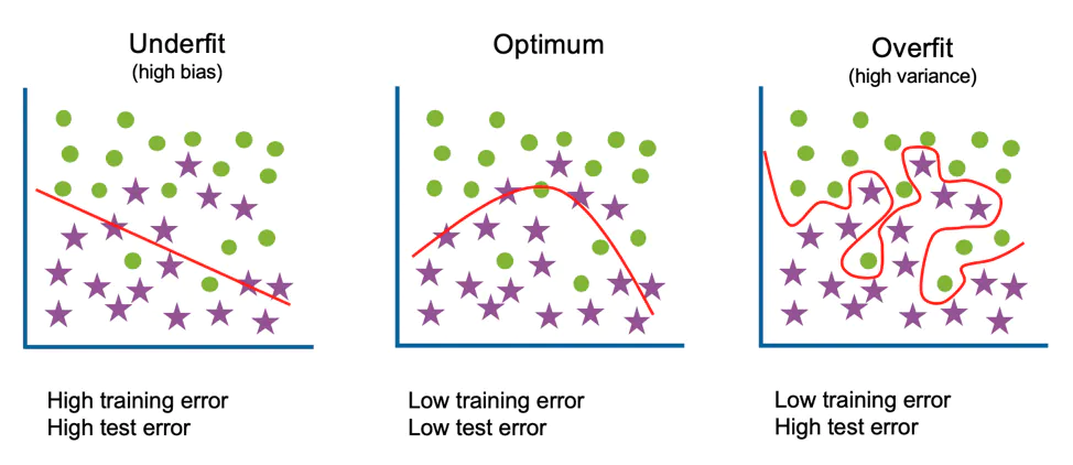
The trained model is called to be overfitted (or overtrained) when it fails to generalise to solve a given problem.

One of examples would be that the model learns to predict exactly the training data and once given a new unseen data drawn from the same distribution it fails to predict the target corrrectly (right plot on Figure 1). Obviously, this is an undesirable behaviour since one wants their model to be "universal" and provide robust and correct decisions regardless of the data subset sampled from the same population.

Hence the solution to check for ability to generalise and to spot overfitting: test a trained model on a separate data set, which is the same¹ as the training one. If the model performance gets significantly worse there, it is a sign that something went wrong and the model's predictive power isn't generalising to the same population.

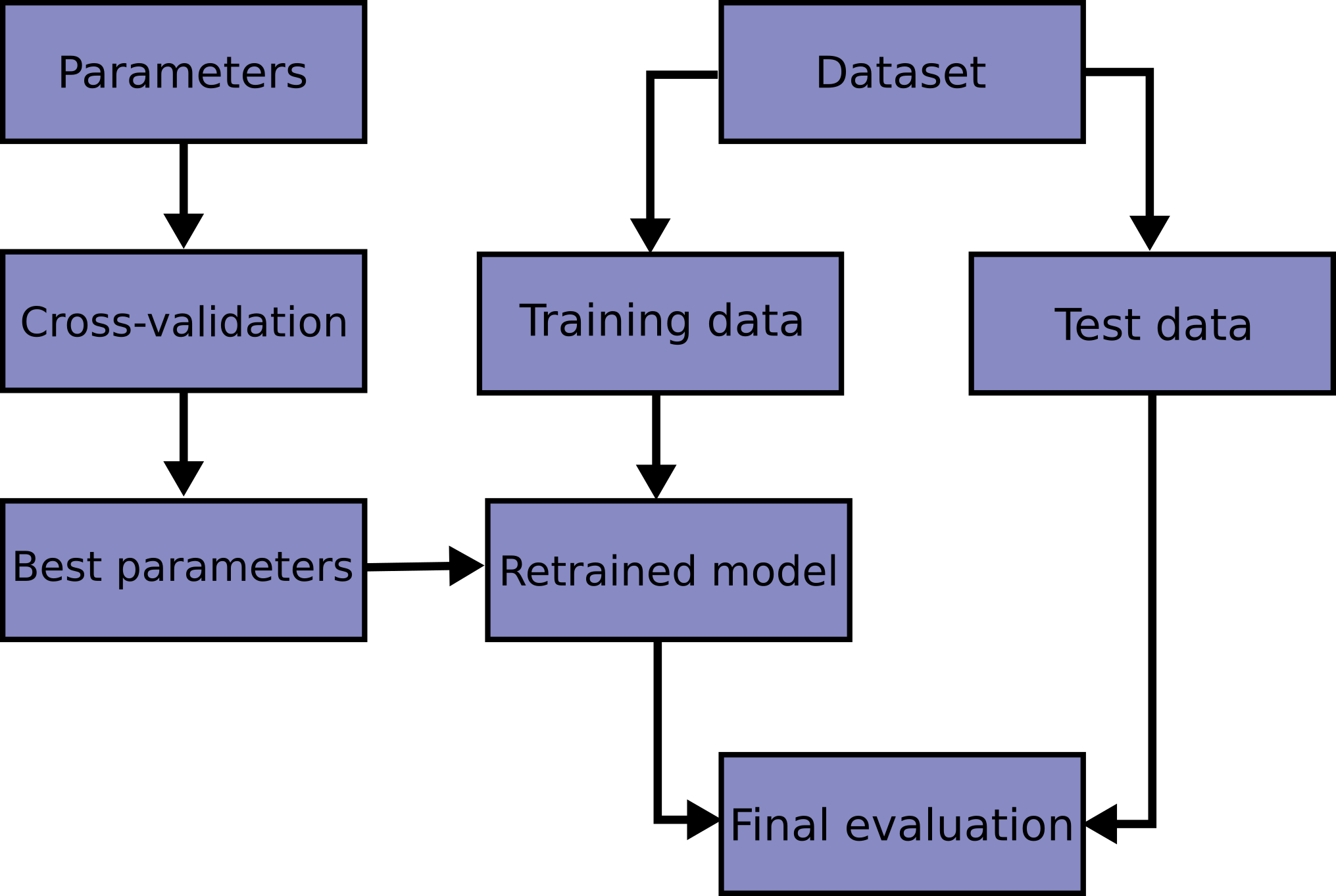
Clearly, the simplest way to find this data set is to put aside a part of the original one and leave it untouched until the final model is trained - this is what is called "test" data set in the first paragraph of this subsection. When the model has been finalised and optimised, this data set is "unblinded" and model performance on it is evaluated. Practically, this split can be easily performed with train_test_split() method of sklearn library.

Lastly, one can also considering to put aside yet another fraction of original data set, what was called "validation" data set. This can be used to monitor the model during the training and more details on that will follow in the overfitting section.

Batches¶

Usually it is the case the training/validation/testing data set can't entirely fit into the memory due to a large size. That is why it gets split into batches (chunks) of a given size which are then fed one by one into the model during the training/testing.

While forming the batches it is important to keep in mind that batches should be sampled uniformly (i.e. from the same underlying PDF as of the original data set).

That means that each batch is populated similarly to the others according to features which are important to the given task (e.g. particles' pt/eta, number of jets, etc.). This is needed to ensure that gradients computed for each batch aren't different from each other and therefore the gradient descent doesn't encounter any sizeable stochasticities during the optimisation step.²

Lastly, it was already mentioned that one should perform preprocessing of the data set prior to training. However, this step can be substituted and/or complemented with an addition of a layer into the architecture, which will essentially do a specified part of preprocessing on every batch as they go through the model. One of the most prominent examples could be an addition of batch/group normalization, coupled with weight standardization layers which turned out to sizeably boost the performance on the large variety of benchmarks.

Training weights¶

Next, one can zoom into the batch and consider the level of single entries there (e.g. events). This is where the training weights come into play. Since the value of a loss function for a given batch is represented as a sum over all the entries in the batch, this sum can be naturally turned into a weighted sum. For example, in case of a cross-entropy loss with y_pred, y_true, w being vectors of predicted labels, true labels and weights respectively:

def CrossEntropy(y_pred, y_true, w): # assuming y_true = {0, 1}
    return -w*[y_true*log(y_pred) + (1-y_true)*log(1-y_pred)]

It is important to disentangle here two factors which define the weight to be applied on a per-event basis because of the different motivations behind them:

• accounting for imbalance in training data
• accounting for imbalance in nature

Imbalance in training data¶

The first point is related to the fact, that in case of classification we may have significantly more (>O(1) times) training data for one class than for the other. Since the training data usually comes from MC simulation, that corresponds to the case when there is more events generated for one physical process than for another. Therefore, here we want to make sure that model is equally presented with instances of each class - this may have a significant impact on the model performance depending on the loss/metric choice.

To account for this type of imbalance, the following weight simply needs to be introduced according to the target label of an object:

train_df['weight'] = 1
train_df.loc[train_df.target == 0, 'weight'] /= np.sum(train_df.loc[train_df.target == 0, 'weight'])
train_df.loc[train_df.target == 1, 'weight'] /= np.sum(train_df.loc[train_df.target == 1, 'weight'])

Alternatively, one can consider using other ways of balancing classes aside of those with training weights. For a more detailed description of them and also a general problem statement see imbalanced-learn documentation.

Imbalance in nature¶

The second case corresponds to the fact that in experiment we expect some classes to be more represented than the others. For example, the signal process usually has way smaller cross-section than background ones and therefore we expect to have in the end fewer events of the signal class. So the motivation of using weights in that case would be to augment the optimisation problem with additional knowledge of expected contribution of physical processes.

Practically, the notion of expected number of events is incorporated into the weights per physical process so that the following conditions hold³:

As a part of this reweighting, one would naturally need to perform the normalisation as of the previous point, however the difference between those two is something which is worth emphasising.